


This post covers some basic procedures for downloading and plotting financial data in the R programming language.
Before starting
- It is highly recommended to work with the IDE RStudio for R.
- For aesthetic reasons, the package ‘ggplot2’ will be used for the data visualization process. The package ‘tidyr’ will also be required. To download, run the following code in the RStudio’s console:
install.packages('ggplot2') install.packages('tidyr') - It is necessary to locate the financial data of your interest within an online database (suggested online database here) with an API that allows to download the data set. In this post the USD/EUR, SGD/EUR and CHF/EUR exchange rates will be used as an example, obtained from the European Central Bank (ECB) database in Quandl. The use of other databases may need some adjustments to the code presented in this post.
Code…
Defining the time interval
First thing to do is to identify the time interval for the financial data. This will be stored as a vector named inter.t. The function Sys.Date() gives the actual date registered in your system. As it can be seen, in this example the time interval is one year long (365 days).
# time interval
 inter.t <- c((Sys.Date()) - 365, (Sys.Date()))
# libraries
library(ggplot2)
require(tidyr)
Downloading, reading and manipulating the data
We proceed to indicate the “links” for downloading the data. Note that Quandl’s R package can be used in this step.
- url: vector containing the urls for the download.
- nam: vector for storing the names of the “to be downloaded” data as .csv
- variables: vector containing the name of the financial data.
# URLs for downloading data:
url <- numeric(); nam <- numeric();
variables <- c("EURUSD", "EURSGD", "EURCHF")

# exchange rate USD per EUR
url[1] <- paste("https://www.quandl.com/api/v3/datasets/ECB/EURUSD.csv?start_date=",
 inter.t[1], "&end_date=", inter.t[2]); nam[1] <- "eurousd.csv"

# exchange rate SGD per EUR
 url[2] <- paste("https://www.quandl.com/api/v3/datasets/ECB/EURSGD.csv?start_date=",
 inter.t[1], "&end_date=", inter.t[2]); nam[2] <- "eursgd.csv"

# exchange rate CHF per EUR
 url[3] <- paste("https://www.quandl.com/api/v3/datasets/ECB/EURCHF.csv?start_date=",
 inter.t[1], "&end_date=", inter.t[2]); nam[2] <- "eurchf.csv"
Now the data is actually going to be downloaded into your working directory as a .csv (with the function download.file()). We proceed to read back the data to the environment with read.csv() function in a for loop to avoid writing the instruction for each variable. The order() and as.Date() functions will be used within the same for loop to avoid any data discrepancy.
- le: number of financial variables.
- fin.data: list that contains dataframes (financial data).
- number.data: number of days each financial data has.
le <- length(url); fin.data <- list()

for (i in 1:le) {
 download.file(url[i], nam[i])
 fin.data[[i]] <- read.csv(file = nam[i], header = TRUE, sep = ",", na.strings = TRUE)
 fin.data[[i]] <- fin.data[[i]][order(fin.data[[i]][, 1]), ]
 fin.data[[i]][, 1] <- as.Date(fin.data[[i]][, 1])
 colnames(fin.data[[i]]) <- c("Date", "Value", rep("Value", ncol(fin.data[[i]])-2))
}
names(fin.data) <- variables

# general information about the database
number.data<- lapply(fin.data, nrow)
number.data
The list number.data has the number of observations (daily rates) we have for the exchange rates. A general view of the data for each rate can be done with the head() function.
lapply(fin.data, head)
So now we have the financial data in a list named fin.data. Inside this list there are three dataframes, each one containing the historical information (date and value) of an exchange rate. Furthermore, in the dataframe we can find two columns. The first one being Date (object class Date) and the other being Value (object class numeric).
This particular arrangement of the data is quite intuitive and useful. It can be handy while trying to manipulate data in order to do operations or analysis. Nevertheless, in the following step we are going to create a general dataframe, another useful way to store this kind of data.
- gen.findat : dataframe containing the financial data
- dff: an auxiliary variable.
gen.findat <- data.frame(Date = character(0), Exchange.rate = character(0), Value = numeric(0))
for (i in 1:le){
 dff <- gather(fin.data[[i]], Exchange.rate, Value, -Date)
 dff$Exchange.rate <- rep(variables[i], nrow(dff))
 gen.findat <- rbind(gen.findat, dff)
}
Plotting
Once having done all the previous code, plotting the exchange rates will be quite easy.
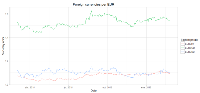
ggplot(gen.findat, aes(x = Date, y = Value, group = Exchange.rate)) +
 geom_line(aes(colour = Exchange.rate), size = 0.8) +
 ggtitle("Foreign currencies per EUR") +
 ylab("Monetary units") +
 theme_light()
Result
At the end we are left with a messy environment and some useful variables. As it has been said before, the variables of interest are the ones that contain the financial data. In this case fin.data and gen.findat. Feel free to clean the environment and leave the variables you want.
The package gglpot2 comes with many editing options. I encourage you to explore them and make a more elegant presentation for the plots.
If you consider that there is a better way of doing a process shown in this post, feel free to mention it in the comments. I will be glad to read your recommendations, it’s always good to learn from other perspectives.
You can download this code or others in github.
For writing readable code, check the Google’s R Style Guide here.
